Author: Wyu-Cnk

Preface

Recently, while playing Turing Complete, I made my way through level after level until I reached Robot Racing. Upon seeing the map

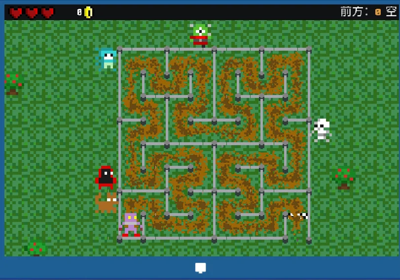
for someone who took Fractal Geometry as an elective, this is nothing but the familiar Hilbert Curve! An old friend! So, I resurrected my long-dormant memories related to fractal geometry, used the concept of fractals to initially implement the corresponding assembly code, and passed the level. Just as I was feeling smug and was checking online how others approached this level, I came across this article: Turing Complete Robot Racing Level - Pure Assembly 60-Byte Achievement Commemoration. Only then did I learn there's an achievement that requires clearing the level with assembly code within 64 bytes, and this article achieved it using a very concise and clever method.

My brother and I discussed and studied the principles of this method together. Now we both understand it and exclaimed "Wow! ". The method in the article essentially also uses the idea of fractals, but the author only gave two simple statements: "It's easy to notice there's an obvious recursive pattern" and "Note that r1 and r2 can be merged and optimized," leaving many talented individuals stumped, as if the author could see through the essence of this method at a glance and thought it was too simple to elaborate on (this_is_what_a_pro_looks_like.jpg). Later, inspired by this article, I also achieved the "Little Machine Runs Fast" achievement. This article will explain, in as plain and understandable language as possible, the approach of using the fractal concept to pass the Robot Racing level and achieve the "Little Machine Runs Fast" achievement, for readers who have or haven't learned about Turing Complete and fractals. It will also provide the assembly code implementing this approach.

Turing Complete

"Turing Complete" is a circuit simulator game that was released on Steam in 2021. In this game, players can build a computer from scratch and program it. While solving puzzles, players will learn knowledge ranging from basic logic gates to complex components like arithmetic units and memory. Following this path, they will ultimately learn how to construct a complete processor architecture. After completing all main levels, players will gain a deeper understanding of the specific connections between processor architecture, assembly language, and electronic components. Players will also learn how concepts common in high-level programming languages, such as conditional statements, loops, and functions, are specifically implemented at the assembly and hardware level. In this article, readers do not need to focus on circuit details; they only need to pay attention to the fractal thought embodied in the algorithm and how to cleverly simplify the algorithm.

Machine Race is a level in the final chapter Assembly Challenge. It requires players to use assembly code to output instructions controlling a robot to move out of a maze. The "Little Machine Run" achievement requires the assembly code written by the player to be as short as possible. The achievement can only be obtained if the code byte count does not exceed 64.

Fractals and Hilbert Curves

A fractal is typically defined as "a rough or fragmented geometric shape that can be split into parts, each of which is (at least approximately) a reduced-size copy of the whole¹", possessing the property of self-similarity. The most common example is a snowflake. In the "Machine Race" challenge, the maze path the robot navigates happens to be a classic type of fractal in fractal geometry: the Hilbert curve. The Hilbert curve is a space-filling curve that can fill a square plane, proposed by David Hilbert in 1891. A curve $H_n$ is called a Hilbert curve if it satisfies the following properties:

1. $H_0$ is the center point of the square.
2. Scale $H_n$ uniformly to $\frac{1}{4}$ of its original size, denoted as $H^{\prime}_n$. Let $s_n$ be the point of $H^{\prime}n$ closest to the bottom-left corner, and $t_n$ be the point closest to the bottom-right corner. $H{n+1}$ is generated by connecting the curves as follows:
   1. Divide the square into $2\times2$ smaller squares.
   2. Let the bottom-left smaller square be $H^{\prime}_n$ rotated $90\degree$ clockwise.
   3. Let the top-left and top-right smaller squares be $H^{\prime}_n$.
   4. Let the bottom-right smaller square be $H^{\prime}_n$ rotated $90\degree$ counter-clockwise.
   5. Connect $s_n$ of the bottom-left square to $s_n$ of the top-left square.
   6. Connect $t_n$ of the top-left square to $s_n$ of the top-right square.
   7. Connect $t_n$ of the top-right square to $t_n$ of the bottom-right square.

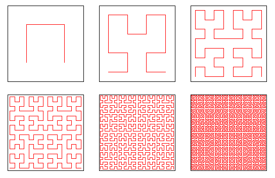
It can be rigorously proven that as $n\rightarrow\infty$, $H_n$ becomes dense in the square, meaning it will fill the entire square plane.

If the square is divided into $2^n\times2^n$ smaller squares, it is easy to see that $H_n$ has the following properties:

1. $H_n$ passes through the center point of all smaller squares, and each smaller square is visited only once.
2. There is at most one connecting line between two adjacent smaller squares.
3. There is no connecting line between two non-adjacent smaller squares.
4. $H_n$ is a polyline (折线) with its two endpoints located at the center points of the bottom-leftmost and bottom-rightmost smaller squares.
5. $H_n$ is non-directional.
6. $H_n$ is symmetric about the vertical centerline.

Main Content

Directed Hilbert Curve

Although the maze's path is a Hilbert curve, there is actually a slight difference. $H_n$ is undirected, but the maze path has a direction—it must go from the starting point in the lower-left corner to the endpoint in the lower-right corner. Therefore, we need to define a directed Hilbert curve by modeling it after the definition of $H_n$.

We denote $\hat{H}_n$ as a directed Hilbert curve if $\hat{H}_n$ satisfies the following properties:

1. $\hat{H}_0$ is the center point of the square.
2. Scale $\hat{H}_n$ down to $\frac{1}{4}$ of its original size, denoted as $\hat{H}^{\prime}_n$. Let the starting point of $\hat{H}^{\prime}_n$ be $\hat{s}_n$ and the endpoint be $\hat{t}n$. $\hat{H}{n+1}$ is generated by connecting as follows:
   1. Divide the square equally into $2\times2$ smaller squares.
   2. Let the smaller square in the lower-left corner be $\hat{H}^{\prime}_n$ with its path reversed and rotated $90\degree$ clockwise.
   3. Let the smaller squares in the upper-left and upper-right be $\hat{H}^{\prime}_n$.
   4. Let the smaller square in the lower-right corner be $\hat{H}^{\prime}_n$ with its path reversed and rotated $90\degree$ counterclockwise.
   5. Connect $\hat{s}_n$ in the lower-left square to $\hat{s}_n$ in the upper-left square, with the direction pointing toward $\hat{s}_n$ in the upper-left square.
   6. Connect $\hat{t}_n$ in the upper-left square to $\hat{s}_n$ in the upper-right square, with the direction pointing toward $\hat{s}_n$ in the upper-right square.
   7. Connect $\hat{t}_n$ in the upper-right square to $\hat{t}_n$ in the lower-right square, with the direction pointing toward $\hat{t}_n$ in the lower-right square.

Here, path reversal means changing the path from its original start-to-end direction to an end-to-start direction. The reason for performing path reversal is that when splicing paths, the endpoint of the previous path must connect to the starting point of the next path to form a new continuous path. Without path reversal, you might end up with "start-to-start" or "end-to-end" connections, which would not produce a valid new path.

If the square is divided equally into $2^n\times2^n$ smaller squares, it is easy to see that $\hat{H}_n$ and $H_n$ share many similar properties:

1. Starting from the starting point, $\hat{H}_n$ passes through the center points of all smaller squares, each smaller square only once, and then reaches the endpoint.
2. Between any two adjacent smaller squares, there is at most one path.
3. Between any two non-adjacent smaller squares, there is no path.
4. The starting point and endpoint of $\hat{H}_n$ are located at the center points of the bottom-left and bottom-right smaller squares, respectively.
5. $\hat{H}_n$ is directed, pointing from the starting point to the endpoint.
6. Reversing the path of $\hat{H}_n$ is equivalent to performing a left-right mirror flip of $\hat{H}_n$.

Property 6 is particularly important, as it is determined by the left-right symmetry of $H_n$: if a path is left-right symmetric when its direction is ignored, then reversing the path is equivalent to performing a left-right mirror flip on the path. This property also means that this operation can be handled using a more convenient method.

Generating Maze Paths

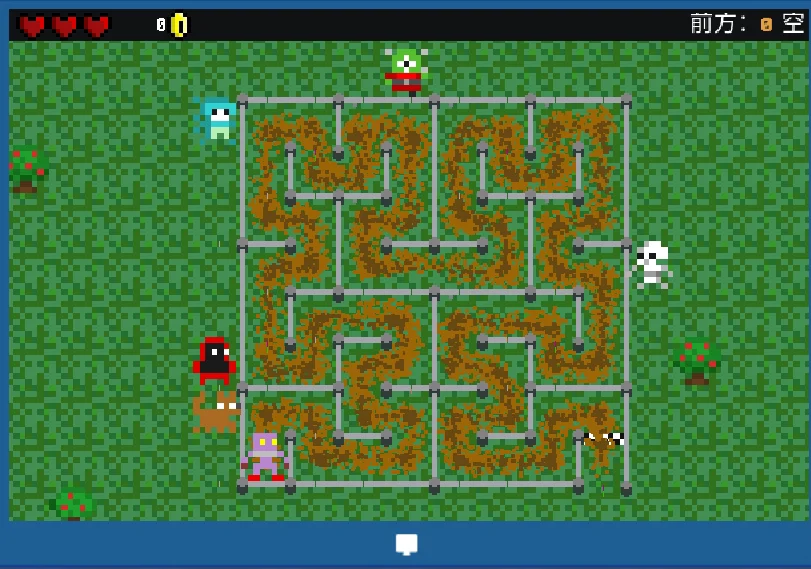
It is easy to see that the maze path is essentially $\hat{H}_3$. If represented using the given instructions, $\hat{H}_3$ is expressed as follows: $$ 301 & 0 & 032 & 3 & 032 & 2 & 123 \ 3 & \ 032 & 3 & 301 & 0 & 301 & 1 & 210 \ 0 & \ 032 & 3 & 301 & 0 & 301 & 1 & 210 \ 1 & \ 123 & 2 & 210 & 1 & 210 & 0 & 301\ $$ To represent the path more vividly, let's denote the path as Instruction 1$\rightarrow$ Instruction 2$\rightarrow\dots\rightarrow$ Instruction $m$, for example, $1\rightarrow2\rightarrow3$. Let $h(n)$ be the path representation of $\hat{H}_n$. Then based on the generation method 2~7 of $\hat{H}_n$, we can derive the generation method for $h(n)$ (note the order of the paths here for sequential output later):

1. $h(1)=3\rightarrow0\rightarrow1$;
2. $h(n+1)=f(h(n))\rightarrow3\rightarrow h(n)\rightarrow0\rightarrow h(n)\rightarrow1\rightarrow g(h(n))$,

where $f$ is the operation that flips the path horizontally and then rotates it $90\degree$ clockwise, and $g$ is the operation that flips the path horizontally and then rotates it $90\degree$ counterclockwise. To define the overall operation on the path, it suffices to define the specific operation for each step of the path. Therefore, only the specific definitions for each step of $f$ and $g$ are provided: $$ f(x)=\begin{cases} 3, & x=0 \ 2, & x=1 \ 1, & x=2 \ 0, & x=3 \end{cases} \quad ,g(x)=\begin{cases} 1, & x=0 \ 0,& x=1 \ 3, & x=2 \ 2, & x=3 \end{cases} \quad. $$ For example, $f(h(1))=f(3\rightarrow0\rightarrow1)=0\rightarrow3\rightarrow2$, and $g(h(1))=g(3\rightarrow0\rightarrow1)=2\rightarrow1\rightarrow0$. Thus, for any given positive integer $n$, we can iteratively generate the corresponding $h(n)$, meaning no matter how many levels the Hilbert maze has, we can solve it with a single formula!

Assembly Code Implementation and Optimization

Before implementing with code, it's necessary to briefly understand what assembly language is. Assembly language is a low-level programming language used for direct interaction with computer hardware. It is a representation of a computer's instruction set architecture, using symbols to represent the machine instructions of a computer. In assembly language, mnemonics replace the operation codes of machine instructions, and address symbols or labels replace the addresses of instructions or operands. Assembly language is closely related to computer hardware; each assembly statement corresponds directly to a low-level machine instruction, operating directly on the computer's registers and memory.

The game "Turing Complete" vividly demonstrates how assembly language operates on registers and memory, but that's not the focus of this section. This section will only extract the relevant principles for explanation.

Bits and Bytes

In the game, a 0-1 switch has only two states: on or off, so binary can be used to represent a 0-1 switch. A bit represents a binary number of length 1, while a byte represents a binary number of length 8, meaning 1 byte = 8 bits. The range of an unsigned 1-byte integer is 0~255. The data mentioned in this section will only be considered within the range of an unsigned 1-byte.

Registers

In the game, a register can be simply understood as a component that can read or write one byte of data. Reading and writing can occur simultaneously.

Instructions

In the game, an instruction consists of 4 bytes: opcode, parameter 1, parameter 2, result address. The opcode corresponds one-to-one with an operation; players can assign aliases to different opcodes within the game to improve the readability of assembly code. Parameters 1 and 2 are register addresses by default, and the program reads the values in the corresponding registers for operation. However, parameters can be specified as immediate values via the opcode, in which case the parameter itself is used for the operation. The result address specifies where the operation's result should be stored (e.g., a register address). For conditional jump operations, the result address refers to the address to jump to when the condition is true. Below is the instruction set that will be used in this section.

add

Syntax

add parameter1 parameter2 result_address

Meaning

Value in the register at result_address = Value in the register at parameter1 + Value in the register at parameter2

Example

add re0 re1 re2 means re2=re0+re1

imme1

Syntax

opcode|imme1 parameter1 parameter2 result_address

Meaning

When executing the opcode, treat parameter1 as an immediate value.

Example

add|imme1 1 re0 re1 means re1=1+re0

imme2

Syntax

opcode|imme2 parameter1 parameter2 result_address

Meaning

When executing the opcode, treat parameter2 as an immediate value.

Example

add|imme2 re0 1 re1 means re1=re0+1

sub

Syntax

sub parameter1 parameter2 result_address

Meaning

Value in the register at result_address = Value in the register at parameter1 - Value in the register at parameter2

Example

sub re0 re1 re2 means re2=re0-re1

and

Syntax

and parameter1 parameter2 result_address

Meaning

Value in the register at result_address = Value in the register at parameter1 & (bitwise AND) Value in the register at parameter2

Example

and re0 re1 re2 means re2=re0&re1

xor

Syntax

xor parameter1 parameter2 result_address

Meaning

Value in the register at result_address = Value in the register at parameter1 ^ (bitwise XOR) Value in the register at parameter2

Example

xor re0 re1 re2 means re2=re0^re1

not

Syntax

not parameter1 _ result_address

Meaning

Value in the register at result_address = ~ (bitwise NOT) Value in the register at parameter1

Example

not re0 0 re1 means re1=~re0

Conditional Jumps

Syntax

conditional_jump_opcode parameter1 parameter2 jump_address

Meaning

If parameter1 and parameter2 meet the condition defined by the conditional jump opcode, then jump to the instruction at jump_address.

Example

label test
// Other code
equl re0 re1 test

Means if re0==re1, then jump to the instruction corresponding to test. Here, label assigns the address of the current instruction to test.

equl

Syntax

equl parameter1 parameter2 jump_address

Meaning

If parameter1 == parameter2, then jump to the instruction at jump_address.

Example

equl re0 re1 test

Means if re0==re1, then jump to the instruction corresponding to test.

call

Syntax

call function_address _ _

Meaning

Call a function, jump to the instruction at function_address.

Example

label fun

Other Code

call fun 0 0

This means calling the `fun` function and jumping to the instruction corresponding to `fun`.

##### return

###### Syntax

```assembly
return _ _ _

Meaning

Jumps to the next instruction after the previously executed call statement.

Example

call fun 0 0
add re0 re1 re2
// Other code
label fun
// Other code
return 0 0 0

After executing the call statement, it jumps to the instruction corresponding to fun. When the return instruction is executed, it jumps back to the next instruction after the previously executed call statement, which is the add instruction.

Code Implementation

The goal of this section is to output $h(n)$ using as little code as possible, as few registers as possible, and the shortest possible runtime. To do this, we first need to process $f$ and $g$. It is easy to verify that $f(x)=(\sim x)&3$ and $g(x)=x\textasciicircum1$. Here, we use the bitwise AND &, bitwise NOT ~, and bitwise XOR ^ operations (按位与 &、按位取反 ~、按位异或 ^). These are all simple logic gate operations, resulting in simple code and fast execution. Moreover, &3 is essentially taking the remainder modulo 4, which can limit the values to a proper range without breaking the one-to-one correspondence between values and instructions.

The following Python code is referenced from: Turing Complete Robot Racing Level - Achieving 60-Byte Pure Assembly Code:

n = 3 
r0 = 0 # Recursion level, h(r0) is the n-r0 level recursion
r1 = 0 # Current path direction

def fill():
  global r0, r1
  if r0 is not n:
    r0 += 1
    r1 = ~r1 # f
    fill() # f(h(n))
    print(r1 & 3, end='') # Instruction 3 for the current level n
    r1 = ~r1 # Backtrack
    fill() # h(n)
    print(r1 & 3, end='') # Instruction 0 for the current level n
    fill() # h(n)
    r1 ^= 1 #g
    print(r1 & 3, end='') # Instruction 1 for the current level n
    fill() # g(h(n))
    r1 ^= 1 # Backtrack
    r0 -= 1 # Backtrack

fill()

The fill() function outputs the sequence for h(n-r0) starting with orientation r1, and the robot's orientation remains r1 after exiting from the endpoint. Note that $f(f(x))=x$ and $g(g(x))=x$, so backtracking in the recursion only requires calling $f$ or $g$ once more.

Translating this into assembly language gives:

label fill
equl|imme2 re0 3 end
add|imme2 re0 1 re0
not|imme2 re1 0 re1 
call fill 0 0
and|imme2 re1 3 out
not|imme2 re1 0 re1
call fill 0 0
and|imme2 re1 3 out 
call fill 0 0
xor|imme2 re1 1 re1 
and|imme2 re1 3 out
call fill 0 0
xor|imme2 re1 1 re1
sub|imme2 re0 1 re0
label end
return 0 0 0

It only requires 60 bytes, achieving the achievement "Robot Racing Sprint"! It uses only two registers, runs very quickly, and is very elegant~

Conclusion

Assembly, as a relatively low-level programming language, possesses a unique charm through its direct manipulation of memory. While optimizing $f$ and $g$, I realized that without a certain "assembly intuition" or "logic gate intuition," it's hard to spot optimization opportunities at a glance. Initially, I used rather clumsy methods to implement these two mappings. It wasn't until I read that article that "makes it obvious" that I had a sudden realization—there was another way to approach this!

Meanwhile, fractals are a fascinating subject, whose beauty and wonder are captivating. Through this article, I hope to inspire more people to discover the beauty of this mathematical treasure. I also encourage players of "图灵完备" (Turing Complete) to strive for the "小机快跑" (Tiny Machine Goes Fast) achievement!

References

Footnotes

1. Mandelbrot Benoit B. 1983. The Fractal Geometry of Nature. [New edition] ed. New York: Freeman. ↩