

Goodbye to NVIDIA CUDA's Monopoly: Running Deep Learning with ROCm on Windows + AMD GPUs — A Hands-On MNIST Handwritten Digit Recognition
Under the Windows + AMD debuff I still managed to compile a ROCm build of PyTorch, and used MNIST, the “Hello World” of the field, to verify it. Using a CNN instead of a tired old fully connected network finally lives up to the GPU’s compute. After 500 batches the loss dropped to 0.03 — for a task this basic, that’s really just checking that the environment works.
目录16 个章节
Preface
I previously described how I wrestled with training models under the stacked debuffs of [Windows + an AMD GPU], and eventually succeeded in compiling a ROCm version of PyTorch, which means I now have the key to enter the world of model training.
Next, to verify whether my self-compiled PyTorch is actually production-capable, we can write a classic MNIST handwritten digit recognition script.
MNIST handwritten digit recognition (28x28 pixels) is known as the “Hello World” of deep learning 😄
This script will include:
- GPU detection.
- Tensor operations (to test the ROCm kernels).
- A model training loop.
Let's go through it step by step.
A Brief Introduction to Neural Networks
A bit of background first.
Neural networks are a core computational model of artificial intelligence inspired by the way neurons connect in the human brain, formed from large numbers of interconnected “artificial neurons” organized into an input layer, hidden layers, and an output layer. By mimicking how the brain processes information, the input layer first receives raw data such as images or text; hidden layers then extract and transform features layer by layer; and finally the output layer produces results such as classification or prediction. Their core strength is the ability to learn autonomously: through a cyclic training process of “forward propagation to compute predictions, backpropagation to adjust connection weights,” model accuracy is continually improved, without any need to manually preset feature rules. Today, neural networks are widely used across every area of life—from face unlock on phones and smart voice assistants, to medical image diagnosis, autonomous driving, and personalized recommendations—and have become a key technology driving AI into real-world use.
I found a pretty good diagram online that clearly shows the structures of various neural networks.
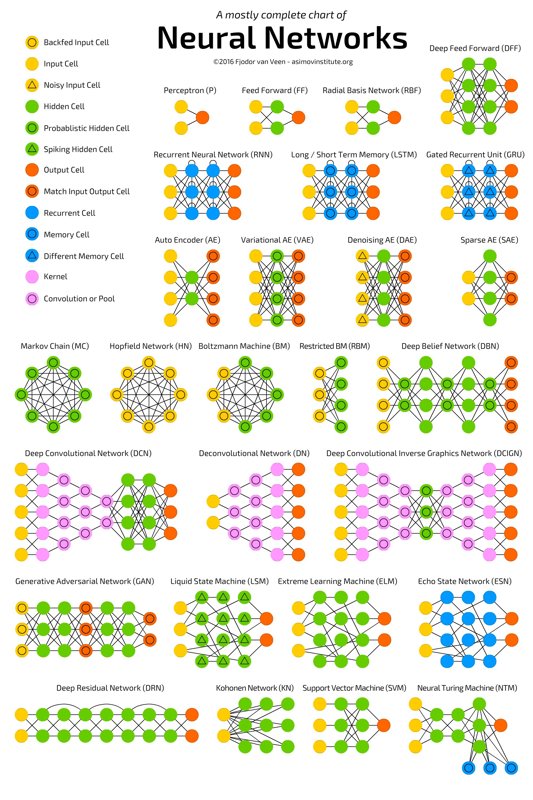
I remember when I first started learning Deep Learning, I read the book Python Neural Network Programming, in which the author taught how to hand-write a neural network with NumPy. Later, another book by the same author, PyTorch Generative Adversarial Networks, implemented a pure fully connected MNIST recognition model in PyTorch. Both belong to feedforward neural networks (Feedforward Neural Network, FNN) (also often called multilayer perceptrons, MLPs).
This article will not use that basic kind of network. Instead it switches to a convolutional neural network (Convolutional Neural Network, CNN)—more specifically, a basic CNN structure combining “convolutional layers + fully connected layers,” which is the most classic and commonly used network type for the MNIST handwritten digit recognition task.
Feedforward Neural Networks (FNN/MLP)
- The most basic neural network structure, no cycles, no feedback, with data flowing in only one “feedforward” direction from input layer→hidden layers→output layer;
- When processing images, a 2D image (such as 28x28 MNIST) is first flattened into a 1D vector (784 elements), then computed through fully connected layers (every neuron is connected to all neurons in the previous layer);
Convolutional Neural Networks (CNN)
- A feedforward-network variant designed specifically for grid-like data (images, speech). The core additions are convolutional layers and pooling layers; they retain the core feedforward logic, but optimize the way features are extracted;
- When processing images they do not flatten immediately; instead a convolution kernel “slides and scans” the image, preserving spatial structure information, then pooling reduces dimensionality, and only then are fully connected layers attached for classification.
Differences
The core differences between the two are whether spatial structure is preserved and the connection pattern: FNN uses full connections + flattening and is suited to non-spatial data; CNN uses local connections + weight sharing and is designed specifically for spatial data such as images.
| Aspect | Feedforward Neural Network (FNN / pure fully connected) | Convolutional Neural Network (CNN) |
|---|---|---|
| Data processing | Flattened directly into a 1D vector, spatial information is lost | 2D spatial structure is preserved; kernels scan to extract features |
| Connection pattern | Fully connected: every neuron is connected to all neurons in the previous layer | Local connections + weight sharing: kernels only connect to local regions; the same kernel parameters are reused |
| Parameter count (MNIST) | Example FNN: 784×128 + 128×64 + 64×10 = 109,328 | Example CNN: conv1 (1×32×3×3) + conv2 (32×64×3×3) + fc1 (9216×128) + fc2 (128×10) ≈ 1,219,624 (looks like more, but on larger images CNN parameters are far fewer than FNN) |
| Feature extraction capability | Can only learn global features; cannot capture local spatial relationships (e.g. the upper and lower loops of the digit “8”) | Hierarchical feature extraction: low-level (edges, lines) → high-level (strokes, digit contours); precisely captures spatial features |
| Robustness to translation / deformation | Poor: a slight shift of the digit is recognized as a different feature | Strong: pooling + convolution make the model insensitive to small shifts and deformations |
| Suitable scenarios | Tabular data, simple classification (non-spatial data) | Images, video, speech, and other grid / sequential spatial data |
Advantages of CNNs
Spatial information is preserved, so feature extraction is more precise
After an FNN flattens a 28x28 image into a 784-dimensional vector, the positional relationship between the top horizontal stroke and the right vertical stroke of the digit “5” is completely scrambled; a CNN’s convolutional layers, by contrast, can “see” these local structures—for example the first conv layer extracts edges, the second extracts stroke combinations—and recognition is ultimately more accurate (on MNIST, FNN accuracy is about 97%, while a simple CNN can reach 99%+).
Higher parameter efficiency, less overfitting
FNN’s fully connected design causes parameters to explode with input size (for example, if you swapped MNIST for 256x256 images, the first FNN layer would have 256×256×128=8,388,608 parameters, whereas CNN conv-layer parameters depend only on the number/size of kernels and are independent of image size); CNN “weight sharing” reuses the same kernel at every position on the image, greatly reducing the number of parameters and lowering the risk of overfitting.
Translation invariance comes naturally
For example, if the digit “3” in MNIST is shifted slightly left or right, an FNN will treat it as a completely different input (because the positions in the flattened vector have changed), whereas a CNN’s convolution + pooling will ignore such small shifts and still recognize it correctly—much more robust.
Installing PyTorch
A quick recap: after PyTorch was successfully compiled in the previous article, there were several artifacts.
Install these three files in order (note: torch must be installed first)
pip install .\torch-2.9.1+rocm7.11.0a20260104-cp312-cp312-win_amd64.whl
pip install .\torchvision-0.24.0+rocm7.11.0a20260104-cp312-cp312-win_amd64.whl
pip install .\torchaudio-2.9.0+rocm7.11.0a20260104-cp312-cp312-win_amd64.whl
GPU Detection and Environment Verification
First activate the virtual environment previously used for ComfyUI; you can also create a new virtual environment. For convenience, I’m simply reusing the earlier virtual environment here.
Use the following code to check the GPU and the environment.
import torch
import torch.nn as nn
import torch.optim as optim
from torchvision import datasets, transforms
from torch.utils.data import DataLoader
import time

# 1. 验证 ROCm 环境
print("="*30)
print(f"PyTorch 版本: {torch.__version__}")
print(f"ROCm 是否可用: {torch.cuda.is_available()}")
if torch.cuda.is_available():
    print(f"当前显卡: {torch.cuda.get_device_name(0)}")
    print(f"AMD 架构: {torch.cuda.get_device_properties(0).gcnArchName if hasattr(torch.cuda.get_device_properties(0), 'gcnArchName') else 'N/A'}")
device = torch.device("cuda" if torch.cuda.is_available() else "cpu")
print(f"正在使用设备: {device}")
print("="*30)
Result:
==============================
PyTorch 版本: 2.9.1+rocm7.11.0a20260104
ROCm 是否可用: True
当前显卡: AMD Radeon RX 6650 XT
AMD 架构: gfx1032
正在使用设备: cuda
==============================
nice! The GPU was detected successfully!
Defining the Model
Digit recognition only needs the simplest CNN model
# 2. 定义一个简单的 CNN 模型
class SimpleCNN(nn.Module):
    def __init__(self):
        super(SimpleCNN, self).__init__()
        self.conv1 = nn.Conv2d(1, 32, 3, 1)
        self.conv2 = nn.Conv2d(32, 64, 3, 1)
        self.fc1 = nn.Linear(9216, 128)
        self.fc2 = nn.Linear(128, 10)

    def forward(self, x):
        x = torch.relu(self.conv1(x))
        x = torch.relu(self.conv2(x))
        x = torch.max_pool2d(x, 2)
        x = torch.flatten(x, 1)
        x = torch.relu(self.fc1(x))
        return self.fc2(x)
Preparing the Data
When I was learning from books before, I even had to go download the data myself. Now the torchvision package ships with the dataset built in. So convenient!
# 3. 准备数据 (MNIST)
transform = transforms.Compose([transforms.ToTensor(), transforms.Normalize((0.1307,), (0.3081,))])
train_dataset = datasets.MNIST('./data', train=True, download=True, transform=transform)
train_loader = DataLoader(train_dataset, batch_size=64, shuffle=True)
This code will load the dataset into the data directory. The result:
 data
 └─ MNIST
    └─ raw
       ├─ train-labels-idx1-ubyte.gz
       ├─ train-labels-idx1-ubyte
       ├─ train-images-idx3-ubyte.gz
       ├─ train-images-idx3-ubyte
       ├─ t10k-labels-idx1-ubyte.gz
       ├─ t10k-labels-idx1-ubyte
       ├─ t10k-images-idx3-ubyte.gz
       └─ t10k-images-idx3-ubyte
Training the Model
The model and data are ready; next we start training
# 4. 初始化模型、损失函数和优化器
model = SimpleCNN().to(device)
optimizer = optim.Adam(model.parameters(), lr=0.001)
criterion = nn.CrossEntropyLoss()

# 5. 开始训练循环
print("\n开始在 AMD GPU 上进行训练测试...")
model.train()
start_time = time.time()

for batch_idx, (data, target) in enumerate(train_loader):
    data, target = data.to(device), target.to(device) # 数据搬运到显存
    optimizer.zero_grad()
    output = model(data)
    loss = criterion(output, target)
    loss.backward()
    optimizer.step()

    if batch_idx % 100 == 0:
        print(f'训练进度: [{batch_idx * len(data)}/{len(train_loader.dataset)}] \t损失: {loss.item():.6f}')

    if batch_idx >= 500: # 只跑 500 个 batch 快速验证
        break

end_time = time.time()
print("\n" + "="*30)
print(f"训练测试完成!耗时: {end_time - start_time:.2f} 秒")
print("="*30)
Results
Running the full code produces output like this
$ python .\mnist.py
==============================
PyTorch 版本: 2.9.1+rocm7.11.0a20260104
ROCm 是否可用: True
当前显卡: AMD Radeon RX 6650 XT
AMD 架构: gfx1032
正在使用设备: cuda
==============================

开始在 AMD GPU 上进行训练测试...
训练进度: [0/60000]     损失: 2.297337
训练进度: [6400/60000]  损失: 0.120939
训练进度: [12800/60000]         损失: 0.053362
训练进度: [19200/60000]         损失: 0.040536
训练进度: [25600/60000]         损失: 0.087424
训练进度: [32000/60000]         损失: 0.036002

==============================
训练测试完成!耗时: 5.61 秒
==============================
Recap
A very good start. Although this task is already far too simple for this GPU, this step has directly opened the door to doing deep learning on AMD cards. I’ll continue to post about using AMD GPUs for deep learning.
In the previous article I saw a fellow reader wanting to use AI image generation to make a cover image of doll-jie 🐶
I’ll set that up once I get the Z-Image workflow running 🐶
_EOF_
Goodbye to NVIDIA CUDA's Monopoly: Running Deep Learning with ROCm on Windows + AMD GPUs — A Hands-On MNIST Handwritten Digit Recognition
- 本文作者:
- 程序设计实验室
- 版权声明:
- 本博客所有文章除特别声明外,均采用 BY-NC-SA 许可协议。转载请注明出处!
相关文章
Windows + AMD 显卡,终于能用 PyTorch 炼丹了
Windows+AMD+ROCm+PyTorch这地狱级组合居然跑通了。无非是用了官方ROCm和保守的PyTorch 2.9.1,避开新版本那些破事。下一步?总算能试试炼丹和AI画图了。
2026-05-09 · ROCm · 约 1 分钟
AMD显卡也能畅玩AI画图!ROCm+ComfyUI部署全指南
用StabilityMatrix在AMD显卡上部署ComfyUI,总算让ROCm派上点正经用场。可视化工作流比早期那堆破烂配置界面强多了,虽然启动时还得手动补依赖。看着GPU利用率拉满生成图像,这才算没白折腾。
2026-05-09 · ROCm · 约 1 分钟
ROCm on Windows 性能排查:RX 6650 XT 跑 PyTorch,为什么加速不明显?
自编译折腾半天,加速不到2倍?小模型+Windows+gfx1032非官方支持,能有这个速度算给面子了。别指望生产环境,当实验玩具玩吧。
2026-05-09 · ROCm · 约 1 分钟
Windows + AMD ROCm + PyTorch:debuff拉满的6650xt A卡炼丹折腾经历
用6650XT在Windows上跑PyTorch?AMD官方都不支持这卡,还得自己编译ROCm。折腾一晚上环境变量和编译错误,结果连个wheel都没生成出来。所以为什么非要在Windows上给A卡炼丹?
2026-05-09 · ROCm · 约 1 分钟
讨论
共 0 条加载评论中…